Frequency distributions

A frequency distribution is a tabular representation of data showing the number of times each observation appears in the dataset. In visual representations, such as histograms, the x-axis typically displays the observed values, while the y-axis represents their corresponding frequencies, showing how often each value occurs. 📅📝

For example, suppose you have collected data on a proficiency test for Class A, in which there are 15 students. These are their scores:

## Load pakcages:

library(tidyverse) 
library(DT) ## For tables
library(DescTools) ## use Mode function

### Create dataset for our proficiency test:

scores <- c(75, 77, 79, 79, 81, 82, 82, 85, 85, 85, 85, 87, 89, 89, 91)

data <- data.frame(
  "Student" = c("Martha", "Fina", "Carol", "Therese", "Bob", "Frank", "Grace", "Henry", "Isabel", "Jack", "James", "Joanna", "Alice", "Esther", "Paola"),
  "Scores" = scores)

### Display table:
DT::datatable(data, options = list(pageLength = 5))

Now, let’s plot a histogram to visualize our frequency distribution:

### Visualize as a histogram: 
## w/ Base R: hist(data$Scores)

## w/ ggplot2:
data %>% 
  ggplot(., aes(x = Scores)) +
  geom_histogram(binwidth=2, boundary= -0.35,
                fill = "skyblue", color = "black") +
  scale_x_continuous(breaks = scores, labels = scores) +
  labs(title = "Distribution of Scores",
       x = "Scores", y = "Frequency") +
  theme_minimal()

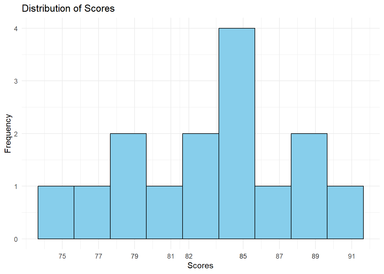
In the histogram above, it is possible to see that each bar represents how many times an observation (i.e, a score) has occured in the dataset.

Measures of Central Tendency

There are many fundamental issues in statistics that go back to frequency distributions, which I will cover in later posts. Today, I will focus on the three measures of central tendency: the mean, the mode and the median.

The Mean

Even if the mean might not be the best measure to get information about a dataset (a topic that I will cover in later posts), you have probably heard many and many times about it. This might be the most intuitive concept in statistics and it is the sum of the total observations in a dataset divided by its total number of observations (n). In our example, the mean is:

Mean = (75 + 77 + 79 + 79 + 81 + 82 + 82 + 85 + 85 + 85 + 85 + 87 + 89 +89 + 91) / 15 = 83.4

In R, this can be easily done using the base function mean()

## Calculate the mean:
meanProf <- mean(data$Scores)

## Display it
meanProf

## [1] 83.4

The Median

The Median is a more reliable measure of central tendency than the mean, especially if we have extreme values in our dataset (I will cover this soon!). It is the observation that is at the center of our distribution, its middle score. As I will show in a later post, the median splits the data into 50%.

The first step to calculate the median is to ordinate all the observations in the dataset in ascending order. After that, we have to determine the observation that is in the center of the distribution. If our dataset is odd, such as ours, then we just count the total number of observations in the dataset (n), add 1 and then divide the result by 2.

1. Sort the dataset in ascending order: 75 77 79 79 81 82 82 85 85 85 85 87 89 89 91 (ps: you can use sort() for that)

2. Find the middle point:

Middle point: (n + 1)/2
Middle point: (15 + 1)/ 2 = 8

3. Identify the median:

Let’s check the number at the 8th position: 75 77 79 79 81 82 82 85 85 85 85 87 89 89 91

That’s our median!

In R, we just have to use the median() function:

## Calculate Median
medianProf <- median(data$Scores)

## Display it
medianProf

## [1] 85

However, if our dataset is even, there’s one more step to calculate the median. First, we repeat the procedure, but the result will be a non-exact number. As such, we should add up the two observations that are within these values and, then, divide the result by two.

1. Originally, our dataset contained 11 numbers, but let’s take the 11th element out to demonstrate how to calculate the median with an even dataset.

75 77 79 79 81 82 82 85 85 85 85 87 89 89 91

2. Find the middle points:

Middle points: (n+1)/2
Middle points: (14+1)/2 = 7.5

Which are the 7th and the 8th values in our dataset?

75 77 79 79 81 82 82 85 85 85 85 87 89 89

3. In order to get the median, we just have to add them up and then divide their sum by two.

Median = (82 + 85)/2 = 83.5

In R:

## Calculate Median
medianProf <- median(data$Scores[1:14])

## Display it
medianProf

## [1] 83.5

The Mode

Finally, the mode represents the most repeated value in our dataset. That is, the value with the biggest frequency, which displays the highest bars in the histogram. Sometimes, however, there are two values with equal distribution in a dataset, when it happens, this will be a bimodal dataset. It is also possible to have multiple modes in a dataset, which we will call a multimodal one.

In our example, which is the most frequent score ?

Take a look back at the histogram above. The highiest bar represents the score 85, which was observed four times in the dataset. Given that this is the most frequent score and that there isn’t another one with the same frequency, this is, precisely, our mode.

Interestingly, for some strange reason, R does not have a built-in function to calculate the mode. There are, however, plenty of user-based functions on the internet, just pick one that suits you.

### Calculate the Mode
## Create a function (https://www.tutorialspoint.com/r/r_mean_median_mode.htm)

getMode <- function(v) {
  uniqv <- unique(v)
  uniqv[which.max(tabulate(match(v, uniqv)))]
}

## Calculate the Mode
modeProf <- getMode(data$Scores)
## Display it:
modeProf

## [1] 85

## Alternatively, you can use the Mode() function from DescTools:
Mode(data$Scores, na.rm = FALSE)

## [1] 85
## attr(,"freq")
## [1] 4

🐕 In this post, we’ve learned about data distributions and the three measures of central tendency: the mean, the median and the mode.

References:

Field, A., Miles, J., & Field, Z. WHY IS MY EVIL LECTURER FORCING ME TO LEARN STATISTICS?. In: Field, A., Miles, J., & Field, Z. (2012). Discovering statistics using R. SAGE Publications, p. 1-31.