Day #03: Polygons
Day3: plot a map with polygons
By Larissa Cury in R
November 3, 2022
Day3’s category is: Polygons. If you don’t know what a Polygon is, I didn’t know either. Hopefully, the plot suits the challenge. 😅 We’ve made it until #day3 yey! You should be able to access the whole script here 😃
Day3: Polygons
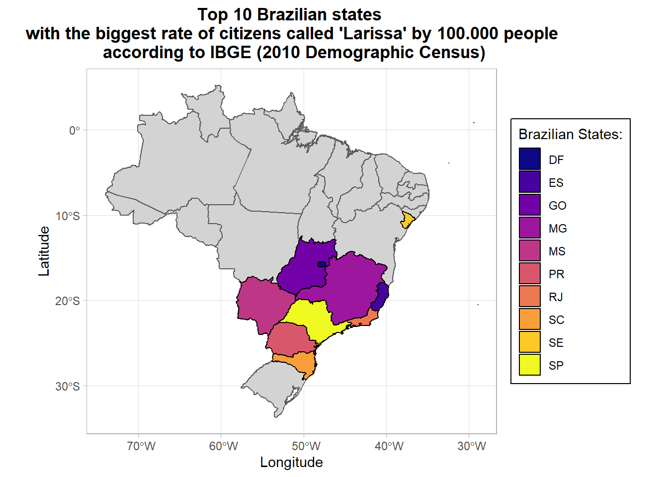
Ploting Brazilian states with the biggest rate of citizens called ‘Larissa’ by 100.000 people
To be pretty honest, I couldn’t think of a linguistic-based topic to plot this map. However, bearing in mind that yesterday I plotted world’s rivers, maybe this is a bit more linguistic-related. I ran out of ideas, so why not plot the top-ten Brazilian states in which my name seems to be the most frequent by a rate of 100.000 people?
I got the data from IBGE (Brazilian Institute of Geography and Statistics). Check out your name too!! 😃

Enough talking! Let’s check the code out?!
Step 1: Load the relevant packages:
### Maps challenge

library(tidyverse)
library(rnaturalearth)
library(rnaturalearthhires)
library(stringr)

# devtools::install_github("AndySouth/rnaturalearthhires")
Step 2: Read tibble:
### Import dataframe:

names <- structure(list(UF = c("SP", "DF", "RJ", "MG", "MS", "ES", "SC",
                      "PR", "GO", "SE"), TAXA = c(235.49, 228.94, 225.44, 202.44, 196.4,
                                                  196.08, 195.73, 189.45, 184.87, 184.81)), row.names = c(NA, -10L
                                                  ), class = c("tbl_df", "tbl", "data.frame"))
### select desired columns:

names <- names %>%
         select(UF, TAXA) %>%
         arrange(desc(TAXA))
Step 3: Filter Brazil and its desired states based on IBGE’s search:
### filter Brazil:

BRA <- ne_states(country = "Brazil", returnclass = "sf")

### select the desired state(s):

States <- BRA %>%
          filter(postal %in% c("SP", "DF", "RJ", "MG", "MS", "ES", "SC", "PR", "GO", "SE")) %>%
          mutate(postal = as.factor(postal))

### I already entered the data in the descending order, the code below is NOT working,
### I don't know why, tho:
# States$TAXA <- names$TAXA
# States1 <- States %>%
#            mutate(States, postal = fct_reorder(postal, TAXA, .fun = identity))
Step 4: Plot it with ggplot2:
library(viridis) ## more colors to ggplot2
## Carregando pacotes exigidos: viridisLite
day3 <- ggplot() +
  geom_sf(data = BRA, fill = "#D3D3D3") + # plot Brazil's map behind it
  geom_sf(data = States, color = "black",  aes(fill = postal)) + # color of the map's border (color); color inside of it (fill)
  # geom_line(data = dat, aes(x = lon, y = lat)) +
  # geom_point(data = dat, aes(x = lon, y = lat, color = Names), size = 3.5, shape = 18) +
  # scale_fill_manual(value = "heat") +
  scale_fill_viridis(option = "C", discrete = TRUE) +
  # scale_fill_brewer(palette="Spectral") +
  theme_light() +
  # geom_text(aes(x = -42, y = -26, label = str_glue("{round(distance/1000, 2)} km"))) +
  labs(x = "Longitude",
       y = "Latitude",
       fill = "Brazilian States:",
       title = "Top 10 Brazilian states \n with the biggest rate of citizens called 'Larissa' by 100.000 people \n according to IBGE (2010 Demographic Census)") +
  theme(legend.position = "right",
        legend.background = element_rect(color = "black"),  # legend block
        axis.text.x = element_text(angle = 0, hjust = 0.4, face = "bold"), # caption
        plot.title = element_text(hjust = 0.5, face = "bold"),
        axis.text.y = element_text(face = "bold"))
Step 5: Visualize it:
Here it goes!
day3
Any suggests are always welcome! My background is in Linguistics, so I’ve never thought I’d be ploting maps, but I’m really enjoying it! Make sure to check the others maps out on twitter using the hashtag #30DayMapChallenge 😆
🐕 Au-au! Today we’ve made our third map using ggplot2 in order to complete the #30DayMapChallenge. Today’s category was Polygons, hopefully we’ve plotted the right plot. We’ve made some research on IBGE and plotted a graph based on IBGE’s search for names. It’s not the best plot ever, but, still, it was really fun to do it, right? Should we say: mission accomplished?! We’ve made it to day 3, yey!! See you soon!